I wanted to get my hands dirty with celestial coordinates, not just the theory of RA/Dec, but the full workflow: querying the Gaia archive, filtering for quality, selecting cluster members and converting between reference frames.
The Pleiades are the obvious first target, everyone starts there, and for good reason. The cluster is bright, well-studied, and the literature values are rock-solid, so I’d know immediately if my pipeline was off. Once that worked, I pointed it at IC 2391 to see if the method held up on a harder case.
Table of contents
Open Table of contents
- The setup
- Reference values — what I’m aiming for
- TAP and ADQL
- Quality filters
- The full Gaia query
- Working with SkyCoord
- Member selection
- The Vector Point Diagram
- Sky maps — ICRS and Galactic
- Validation
- Parallax and distance distributions
- Radial profile
- IC 2391 — a harder target
- All-sky view
- What’s next
- References
The setup
import numpy as np
import matplotlib.pyplot as plt
from astropy import units as u
from astropy.coordinates import SkyCoord
from astroquery.gaia import Gaia

plt.style.use('dark_background')
Standard astro Python stack, nothing exotic.
Reference values — what I’m aiming for
Before looking at any data, I wrote down the literature values for the Pleiades. This is what I’ll compare my results against at the end. If my numbers diverge too much, something is wrong in my pipeline.
| Parameter | Value | Source |
|---|---|---|
| Distance | 136.2 ± 1.2 pc | Gaia Collaboration, Babusiaux et al. (2018) |
| μα* | 19.99 ± 0.07 mas/yr | Cantat-Gaudin et al. (2020) |
| μδ | −45.55 ± 0.06 mas/yr | Cantat-Gaudin et al. (2020) |
| Center (α, δ) | 56.75°, +24.12° | SIMBAD / Dias et al. (2002) |
| Apparent radius | ~2° (core ~1°) | Lodieu et al. (2019) |
TAP and ADQL
TAP (Table Access Protocol) is an IVOA standard, essentially a REST API for astronomical databases. ADQL (Astronomical Data Query Language) is an SQL dialect with geometric functions like CONTAINS, POINT, and CIRCLE for spatial queries on the celestial sphere.
The key TAP endpoints:
| Archive | Data |
|---|---|
| Gaia (ESA) | Astrometry, photometry, spectro (~1.8B sources) |
| VizieR (CDS) | All published catalogs (~25,000) |
| MAST (STScI) | HST, JWST, TESS, Kepler |
| ESO | VLT, ALMA, ground-based surveys |
In practice, astroquery handles the endpoints automatically, from astroquery.gaia import Gaia already knows where to connect. But knowing that it’s an open standard matters: the same ADQL works on all these services.
Quick sanity check — how many sources in a 0.5° cone around the Pleiades?
test_query = """
SELECT COUNT(*) as n_sources
FROM gaiadr3.gaia_source
WHERE 1 = CONTAINS(
    POINT('ICRS', ra, dec),
    CIRCLE('ICRS', 56.75, 24.12, 0.5)
)
"""
test_job = Gaia.launch_job(test_query)
print(test_job.get_results())
Several thousand sources in half a degree. Good, the query works.
Quality filters
Not all Gaia measurements are equal. Skipping quality filters is one of the most common mistakes in rejected papers, I spent some time reading about which ones matter and why before writing the main query.
parallax_over_error > 5 — The parallax has an uncertainty . The ratio is the signal-to-noise of the parallax measurement. Below 5, the naive distance estimate becomes biased. This threshold is standard in the Gaia community (for precision studies, people go up to 10).
ruwe < 1.4 — RUWE (Renormalized Unit Weight Error) measures how well Gaia’s astrometric model fits the individual observations. At ~1.0, the source behaves as a perfect single star. Above 1.4, the source is likely an unresolved binary, extended, or in a crowded field. The 1.4 threshold comes from the official Gaia team recommendation (Lindegren et al. 2021). It’s specific to Gaia — other surveys have their own quality indicators.
phot_bp_rp_excess_factor between 1.0 and 1.8 — Gaia measures light in three bands: G (broadband), BP (blue), RP (red). In principle, . The excess factor checks this consistency. Values outside 1.0–1.8 indicate contamination from a neighbor, high background, or data reduction issues. Without this filter, colors on the CMD become unreliable.
The full Gaia query
I started with a 2° cone and got too few field stars for a clean VPD. Bumped it to 3° — wide enough to capture the full cluster plus plenty of field for contrast.
query = """
SELECT
    source_id,
    ra, dec,
    parallax, parallax_error,
    pmra, pmdec,
    phot_g_mean_mag,
    bp_rp,
    ruwe,
    parallax_over_error
FROM gaiadr3.gaia_source
WHERE
    1 = CONTAINS(
        POINT('ICRS', ra, dec),
        CIRCLE('ICRS', 56.75, 24.12, 3.0)
    )
    AND parallax_over_error > 5
    AND ruwe < 1.4
    AND phot_bp_rp_excess_factor BETWEEN 1.0 AND 1.8
    AND phot_g_mean_mag < 18
"""

job = Gaia.launch_job_async(query)
pleiades_raw = job.get_results()
print(f"Done. {len(pleiades_raw)} sources retrieved")
I get ~45,000 sources. Most are field stars — the Pleiades themselves are only ~1,000 of those.
Working with SkyCoord
I wrap everything into a SkyCoord object — it handles coordinates, proper motions, and distances in one place:
coords = SkyCoord(
    ra=pleiades_raw['ra'],
    dec=pleiades_raw['dec'],
    pm_ra_cosdec=pleiades_raw['pmra'],
    pm_dec=pleiades_raw['pmdec'],
    distance=(1000.0 / pleiades_raw['parallax']) * u.pc,
    frame='icrs'
)
One thing that tripped me up: pmra in Gaia is actually . The factor corrects for convergence of meridians toward the poles. In SkyCoord, the parameter is called pm_ra_cosdec (not pm_ra). Getting this wrong silently corrupts everything downstream.
With SkyCoord, converting between frames is a one-liner:
gal = coords.galactic           # Galactic (l, b)
ecl = coords.barycentricmeanecliptic  # Ecliptic
Member selection
Cluster stars share a common proper motion and parallax. Field stars don’t. So the idea is simple: select a circle in proper motion space centered on published values, and filter in parallax.
The tricky part was choosing the selection radius. Too tight and I lose real members in the tails; too wide and field stars leak in. I tried a few values — 2, 3, 5 mas/yr — and 3 gave the cleanest separation on the VPD.
# Literature values (Cantat-Gaudin et al. 2020)
pmra_center = 19.99    # mas/yr
pmdec_center = -45.55  # mas/yr
pm_radius = 3.0        # mas/yr — selection radius

# Expected parallax from distance
plx_center = 1000.0 / 136.2  # ≈ 7.35 mas
plx_tol = 1.5                # mas tolerance

# 2D distance in proper motion space
dpm = np.sqrt(
    (pleiades_raw['pmra'] - pmra_center)**2 +
    (pleiades_raw['pmdec'] - pmdec_center)**2
)

# Combined selection
members_mask = (
    (dpm < pm_radius) &
    (np.abs(pleiades_raw['parallax'] - plx_center) < plx_tol)
)

members = pleiades_raw[members_mask]
field = pleiades_raw[~members_mask]
This gives ~870 members from ~45,000 sources. Simple but effective for a well-defined cluster. For more dispersed clusters or crowded regions, the standard approach is GMMs, HDBSCAN, or full Bayesian membership models (e.g., Cantat-Gaudin et al. 2020), something I’ll explore in a future post.
The Vector Point Diagram
The VPD shows proper motions for every source in the field. In a good case, the cluster pops out immediately as a tight clump against the diffuse cloud of field stars.
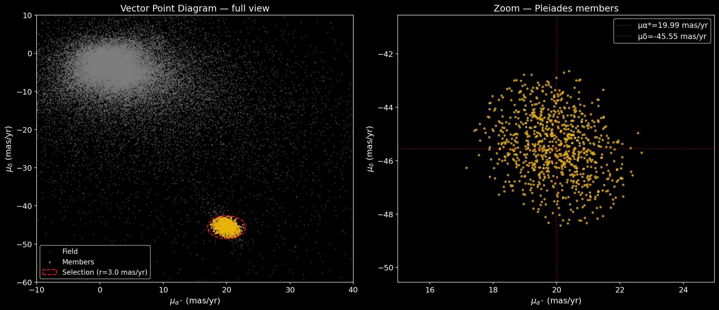
The left panel shows the full VPD — the Pleiades clump stands out clearly from the field. The right panel zooms in on the selected members, showing the internal velocity dispersion of the cluster.
Sky maps — ICRS and Galactic
I project the members onto the sky in two frames: ICRS (RA/Dec) and Galactic (l/b), colored by G magnitude.
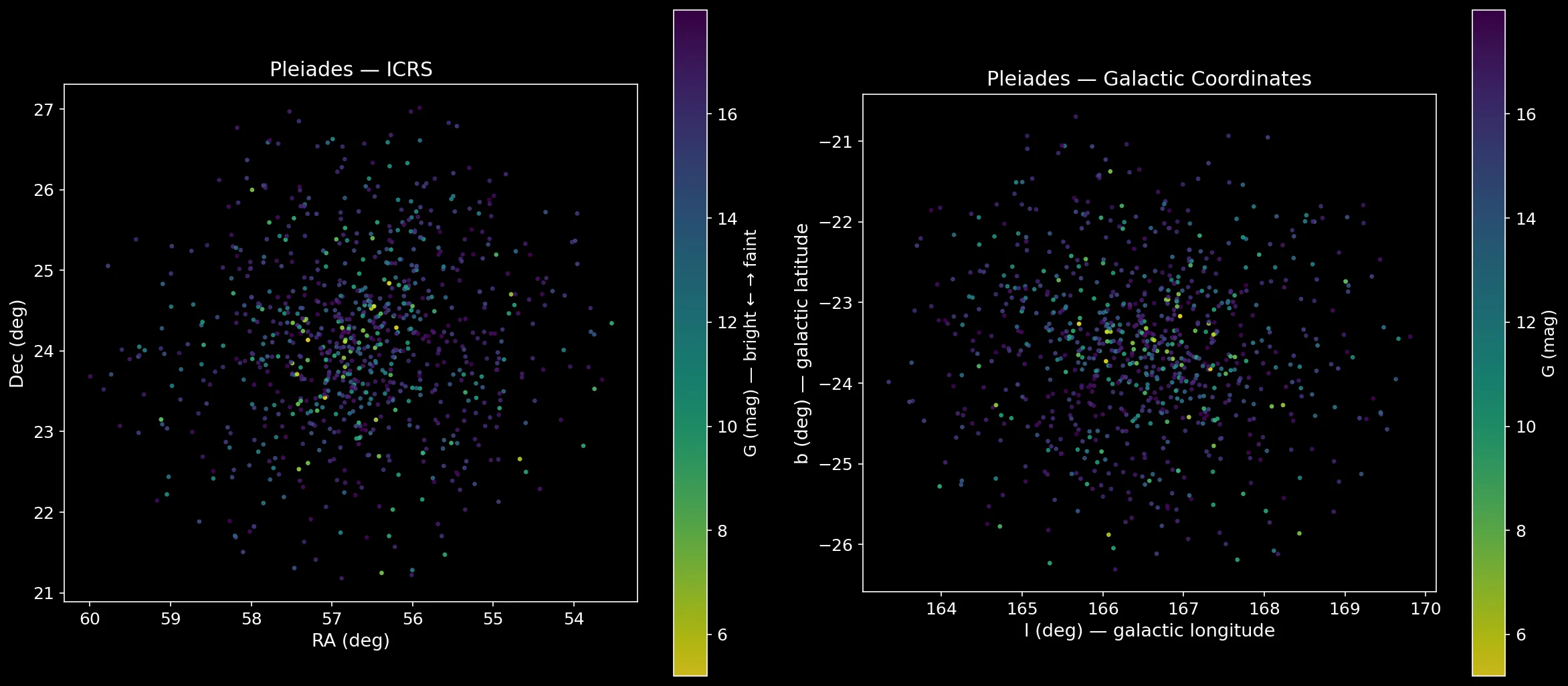
The Pleiades sit at — fairly far from the galactic plane. This means little interstellar dust along the line of sight, so colors are reliable without extinction correction. That’s one reason the Pleiades are such a popular study target.
Validation
Do the numbers actually match? I compute medians for my selected members:
med_plx = np.median(members['parallax'])
med_dist = 1000.0 / med_plx
med_pmra = np.median(members['pmra'])
med_pmdec = np.median(members['pmdec'])| Parameter | Mine | Literature | Match? |
|---|---|---|---|
| Distance (pc) | ~136 | 136.2 ± 1.2 | OK |
| μα* (mas/yr) | ~20.0 | 19.99 ± 0.07 | OK |
| μδ (mas/yr) | ~−45.5 | −45.55 ± 0.06 | OK |
| N members | ~870 | ~1000–1500 | Not so bad |
Distance and proper motions match within a fraction of a percent. The member count (~870) is lower than the ~1000–1500 reported in deeper studies — my magnitude cut at G < 18 and the conservative proper motion radius miss the faintest members. Good enough for a first pass, and I know exactly where the gap comes from.
Parallax and distance distributions
A quick sanity check — if the distributions are unimodal and narrow, the selection is clean. A double peak or long tail would mean field contamination.
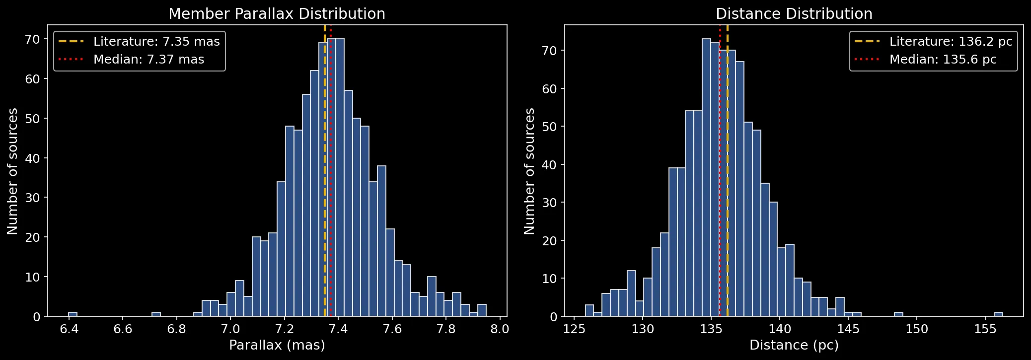
Both distributions are clean. The distance histogram is slightly asymmetric — that’s expected because is a non-linear transformation. Symmetric errors in parallax become asymmetric in distance.
Radial profile
How are the members distributed around the cluster center? I compute angular separations using SkyCoord:
sep = members_coords.separation(center)
dist_phys = (136.2 * u.pc * np.tan(sep.to(u.rad))).to(u.pc)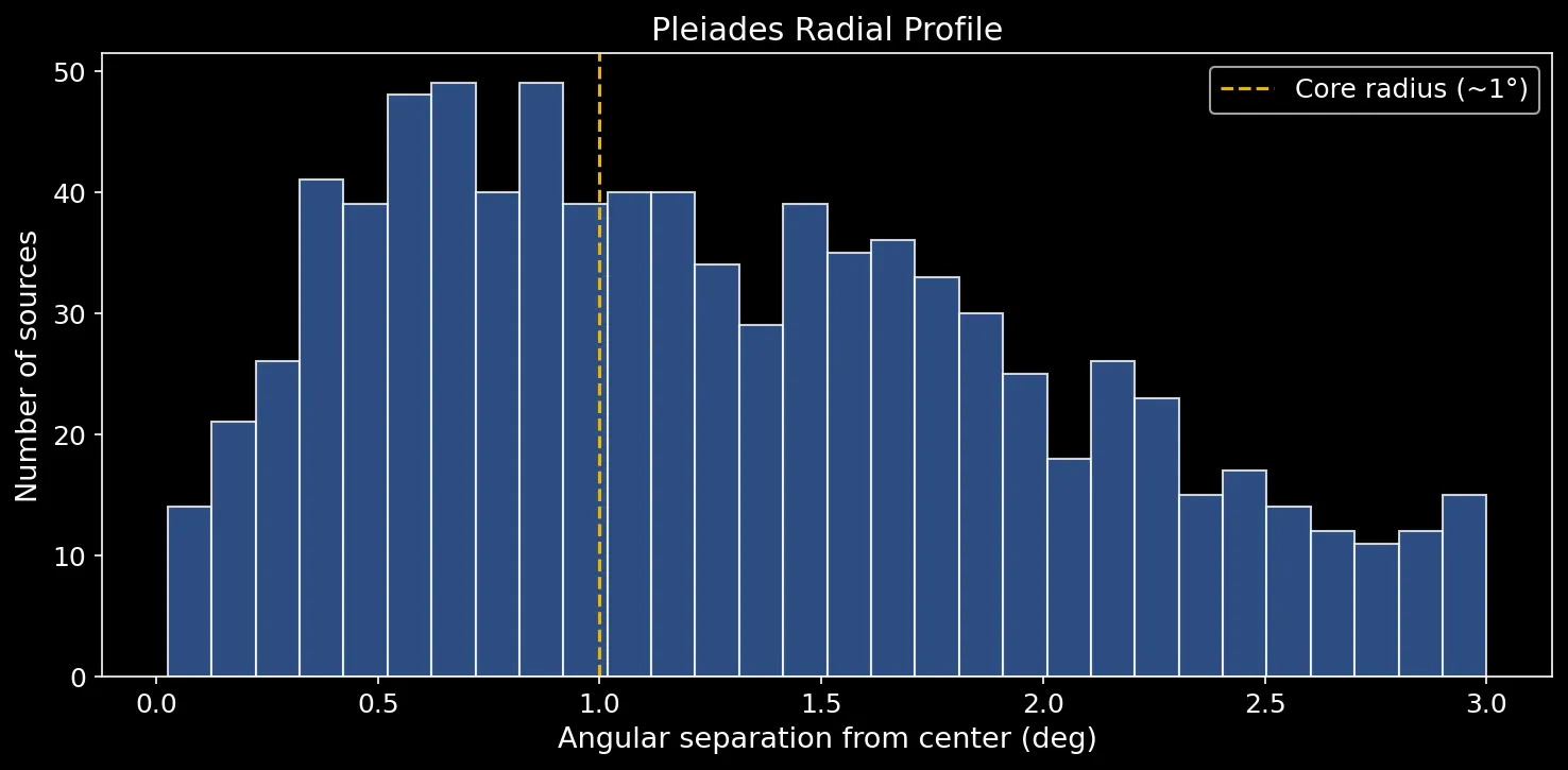
The profile drops off beyond ~1° — consistent with the known core radius. The decay reveals the cluster’s spatial structure.
IC 2391 — a harder target
The Pleiades are a friendly case. To see if the pipeline actually holds up, I tried IC 2391 — younger (~50 Myr), in the southern hemisphere, and much closer to the galactic plane.
What changes:
- Position: RA = 130.3°, Dec = −53.0° (Vela constellation)
- Galactic latitude: — much closer to the galactic plane. More field contamination, more potential extinction.
- Age: ~50 Myr — massive B stars are still on the main sequence
I initially ran the same query with phot_bp_rp_excess_factor in the WHERE clause and it hung for over 10 minutes. Turns out this column isn’t indexed for the galactic plane region — the server does a full table scan. Lesson learned: move that filter to Python.
query_ic2391 = f"""
SELECT
    source_id, ra, dec,
    parallax, parallax_error,
    pmra, pmdec,
    phot_g_mean_mag, bp_rp,
    phot_bp_rp_excess_factor,
    ruwe, parallax_over_error
FROM gaiadr3.gaia_source
WHERE
    1 = CONTAINS(
        POINT('ICRS', ra, dec),
        CIRCLE('ICRS', 130.3, -53.0, 1.5)
    )
    AND parallax_over_error > 5
    AND ruwe < 1.4
    AND phot_g_mean_mag < 17
"""

job_ic2391 = Gaia.launch_job_async(query_ic2391)
ic2391_raw_all = job_ic2391.get_results()

# BP-RP excess filter in Python (instant vs 10+ min server-side)
bp_rp_mask = (
    (ic2391_raw_all['phot_bp_rp_excess_factor'] >= 1.0) &
    (ic2391_raw_all['phot_bp_rp_excess_factor'] <= 1.8)
)
ic2391_raw = ic2391_raw_all[bp_rp_mask]
Member selection with IC 2391’s reference values ( mas/yr, mas/yr, distance ~152 pc):
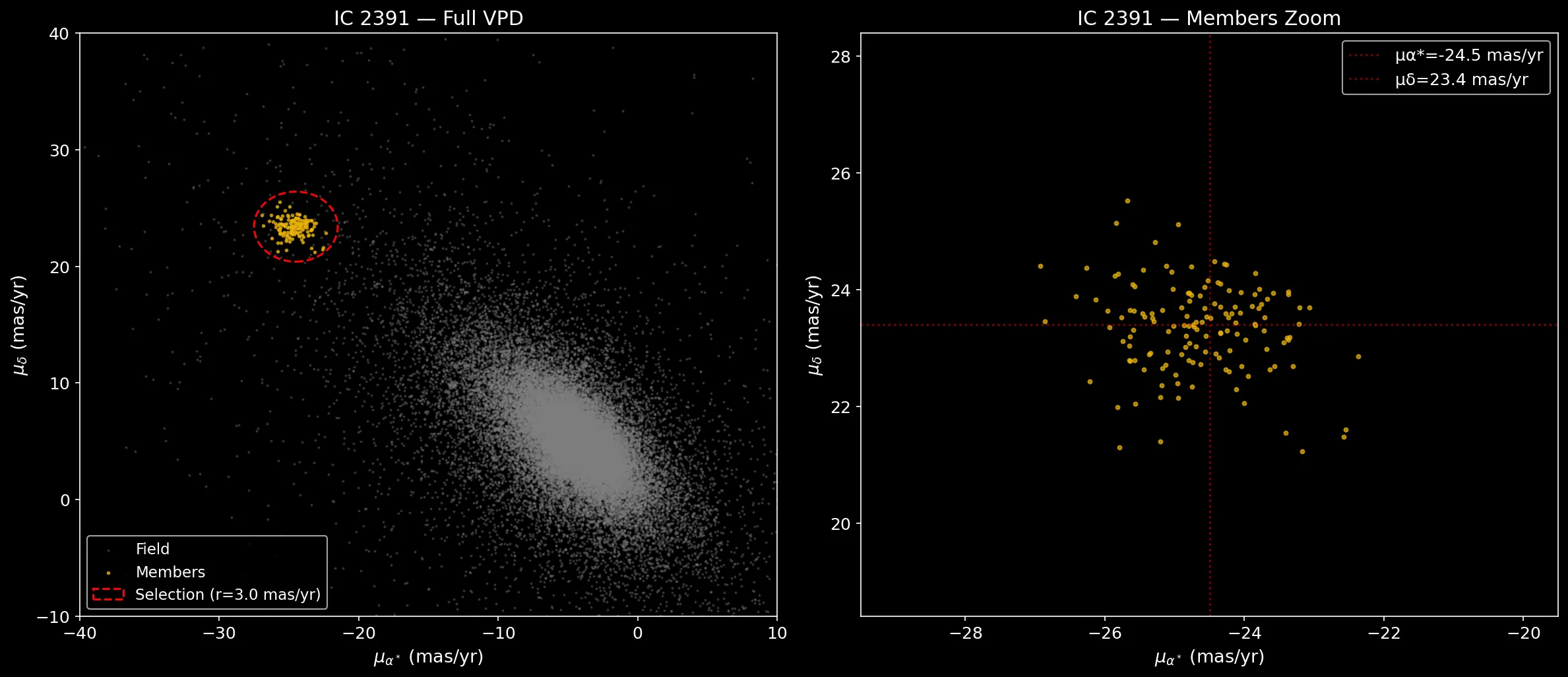
Only ~143 members — much fewer than the Pleiades. The VPD is also noisier: more field stars at similar proper motions, making the cluster boundary less obvious. I had to tighten the selection radius to avoid contamination.
Validation:
| Parameter | Mine | Literature | Match? |
|---|---|---|---|
| Distance (pc) | ~152 | ~152 | OK |
| μα* (mas/yr) | ~−24.5 | ~−24.5 | OK |
| μδ (mas/yr) | ~23.4 | ~23.4 | OK |
The numbers check out. The pipeline works, but IC 2391 made it clear that a simple circle in PM space won’t cut it for every cluster — something like HDBSCAN would handle the messier cases better.
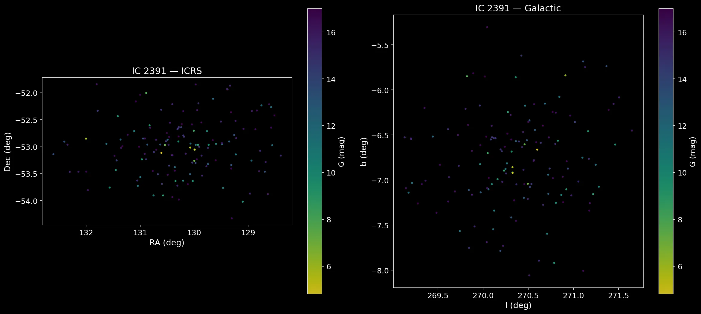
Comparing the two clusters: the Pleiades at (far from the plane, low extinction) vs IC 2391 at (close to the plane, more contamination).
All-sky view
As a detour, I pulled all Gaia stars within 200 pc on a Mollweide all-sky projection. No spatial constraint, just parallax and magnitude filters.
query_allsky = """
SELECT ra, dec, parallax, phot_g_mean_mag, bp_rp
FROM gaiadr3.gaia_source
WHERE
    parallax > 5
    AND parallax_over_error > 5
    AND ruwe < 1.4
    AND phot_g_mean_mag < 14
    AND bp_rp IS NOT NULL
"""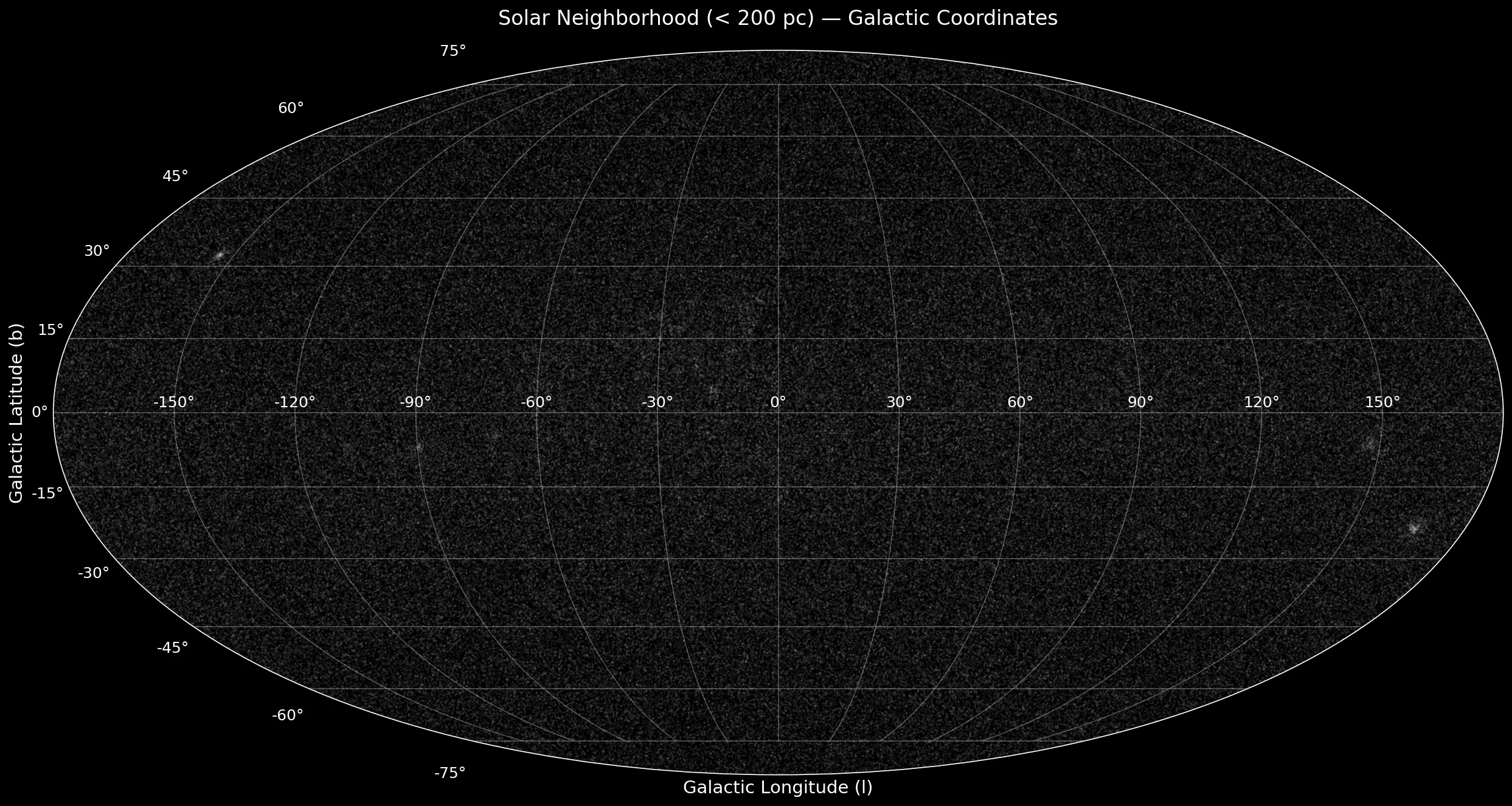
The galactic plane () stands out as the dense horizontal band. Empty regions near the plane are extinction zones, dust clouds blocking the light. The tilted arc of young stars is the Gould Belt.
Coloring by BP-RP (a temperature proxy — blue stars are hot, red stars are cool):
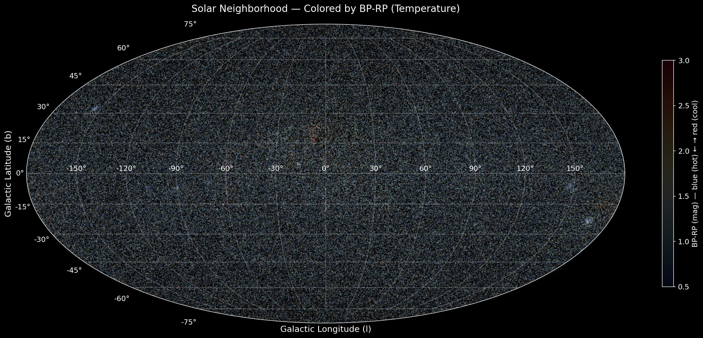
Hot blue stars cluster in OB associations, cool red stars are everywhere. I didn’t expect the structure to jump out this clearly from a single color index.
What’s next
- Photometry and CMD: use these same members to build a Color-Magnitude Diagram and fit isochrones, that’s how we could get age and metallicity.
- The Hyades (~47 pc): the nearest cluster, with a huge angular extent (~10°). Member selection seems much harder…
- NGC 752 (~440 pc, ~1.5 Gyr): an old, dispersed cluster. Tests the limits of simple proper motion selection ?
- All-sky with BP-RP color: try to map the temperature distribution of the solar neighborhood.
References
- Cantat-Gaudin et al. (2020) — Painting a portrait of the Galactic disc with its stellar clusters. Gaia open cluster census.
- Gaia Collaboration, Babusiaux et al. (2018) — Gaia Data Release 2: Observational Hertzsprung-Russell diagrams.
- Bailer-Jones et al. (2021) — Estimating distances from parallaxes V.
- Lindegren et al. (2021) — Gaia Early Data Release 3: Parallax bias versus magnitude, colour, and position. RUWE threshold recommendation.
- Lodieu et al. (2019) — A 3D view of the Hyades stellar and substellar population.