With the Pleiades coordinate pipeline working (previous post), I wanted to go deeper: how bright are these stars, really? And what can brightness alone tell us about their physics? Let’s take a look.
The goal: build a Color-Magnitude Diagram from scratch and see if I can read stellar evolution directly off the plot.
Table of contents
Open Table of contents
- Magnitudes — a 2000-year-old scale
- Apparent vs absolute magnitude
- Same Pleiades, more columns
- Magnitude uncertainties from flux SNR
- Distance modulus
- Gaia’s three bands
- Bolometric luminosity
- Building the CMD
- The turn-off as a clock
- Apparent vs absolute CMD
- Uncertainties on the CMD
- Validation
- What’s next
- References
Magnitudes — a 2000-year-old scale
The magnitude system dates back to Hipparchus (2nd century BCE), who ranked stars from 1st magnitude (brightest) to 6th magnitude (faintest visible to the naked eye). In 1856, Norman Pogson formalized the relationship:
The scale is inverted, smaller magnitudes mean brighter. The Sun sits at , Vega at , and the naked-eye limit is around . Each magnitude step is a factor in flux, and 5 magnitudes = factor 100 in flux, that’s the definition ().
Why logarithmic? Stellar fluxes span between the Sun and Gaia’s faintest targets and the log scale compresses this into a manageable range ( to mag).
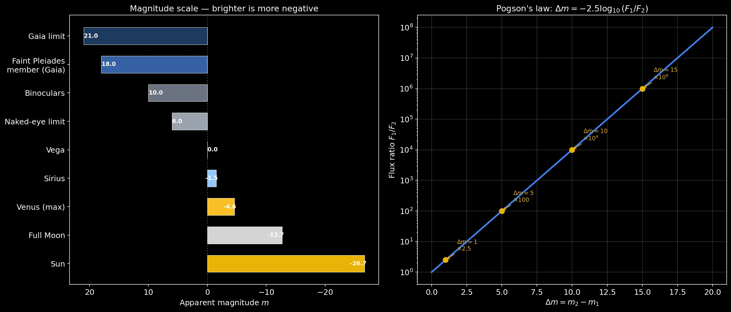
The Sun at , Sirius at , a faint Pleiades member around , almost 45 magnitudes of range. On the right, Pogson’s law: flux ratio vs . On a log scale it’s a straight line, , .
Apparent vs absolute magnitude
The problem with apparent magnitude : it mixes intrinsic brightness and distance. A dim nearby star and a brilliant distant one can look identical. The fix is absolute magnitude , the magnitude an object would have at exactly 10 pc.
The distance modulus connects them:
With Gaia parallax (in mas), pc, so:
For a cluster, all stars are at roughly the same distance, so the distance modulus is a single number that shifts everything vertically:
| Distance modulus | Distance |
|---|---|
| 0 mag | 10 pc |
| 5 mag | 100 pc |
| 5.67 mag | 136 pc (Pleiades) |
| 10 mag | 1,000 pc |
| 15 mag | 10,000 pc |
But, this formula assumes zero extinction (no interstellar dust absorbing light) on the way.. The full version adds : . For the Pleiades at , extinction is negligible (~0.1 mag in G). For clusters embedded in the galactic plane, it becomes the dominant error source.
Same Pleiades, more columns
I start from the same Pleiades members as the previous post, same quality filters, same member selection. Two changes to the query this time: individual BP and RP magnitudes (not just the combined color index), and flux signal-to-noise columns to compute photometric uncertainties.
I also added a parallax BETWEEN 5.0 AND 10.0 pre-filter in the ADQL. This targets the Pleiades distance range (~100–200 pc) directly in the database and cuts the returned data volume dramatically. Without it I was hitting the server row limit on some runs.
query = """
SELECT TOP 5000 source_id, ra, dec, parallax, parallax_error,
       pmra, pmdec,
       phot_g_mean_mag,
       phot_bp_mean_mag,
       phot_rp_mean_mag,
       bp_rp,
       phot_g_mean_flux_over_error,
       phot_bp_mean_flux_over_error,
       phot_rp_mean_flux_over_error,
       ruwe
FROM gaiadr3.gaia_source
WHERE 1 = CONTAINS(
    POINT('ICRS', ra, dec),
    CIRCLE('ICRS', 56.75, 24.12, 3.0)
)
AND parallax BETWEEN 5.0 AND 10.0
AND parallax_over_error > 5
AND ruwe < 1.4
AND phot_bp_rp_excess_factor BETWEEN 1.0 AND 1.8
AND phot_g_mean_mag < 18
"""

for attempt in range(3):
    try:
        job = Gaia.launch_job(query)
        data = job.get_results()
        break
    except Exception as e:
        if attempt < 2:
            print(f"Gaia error (attempt {attempt+1}/3), retrying...")
            time.sleep(5)
        else:
            raise RuntimeError(f"Gaia unavailable: {e}")

# Same member selection as the coordinates post
dpm = np.sqrt((data['pmra'] - 19.99)**2 + (data['pmdec'] + 45.55)**2)
mask = (dpm < 3.0) & (np.abs(data['parallax'] - 7.35) < 1.5)
members = data[mask]
One thing I learned the hard way: Gaia.launch_job_async() was returning intermittent 500 errors from the ESA server. Switching to launch_job() (synchronous) with a retry loop fixed it. The async version is meant for large queries that take minutes, for a few thousand rows, sync seems to be more reliable.
Same ~870 members as before.
Magnitude uncertainties from flux SNR
Gaia doesn’t report magnitude errors directly, it reports flux signal-to-noise ratios. The conversion comes from error propagation on :
where . At SNR = 100, that’s mag. At SNR = 1000, mag.
members['phot_g_mean_mag_error']  = 1.0857 / members['phot_g_mean_flux_over_error']
members['phot_bp_mean_mag_error'] = 1.0857 / members['phot_bp_mean_flux_over_error']
members['phot_rp_mean_mag_error'] = 1.0857 / members['phot_rp_mean_flux_over_error']
I initially looked for phot_g_mean_mag_error columns in the Gaia catalog. They don’t exist, you have to compute them yourself from the flux columns. Not obvious if you’re just browsing the schema.
Distance modulus
First real test: computing the absolute magnitude and distance modulus for every member, then comparing against the published value.
members['abs_g'] = (
    members['phot_g_mean_mag']
    + 5 * np.log10(members['parallax'] / 1000)
    + 5
)
members['dist_mod'] = members['phot_g_mean_mag'] - members['abs_g']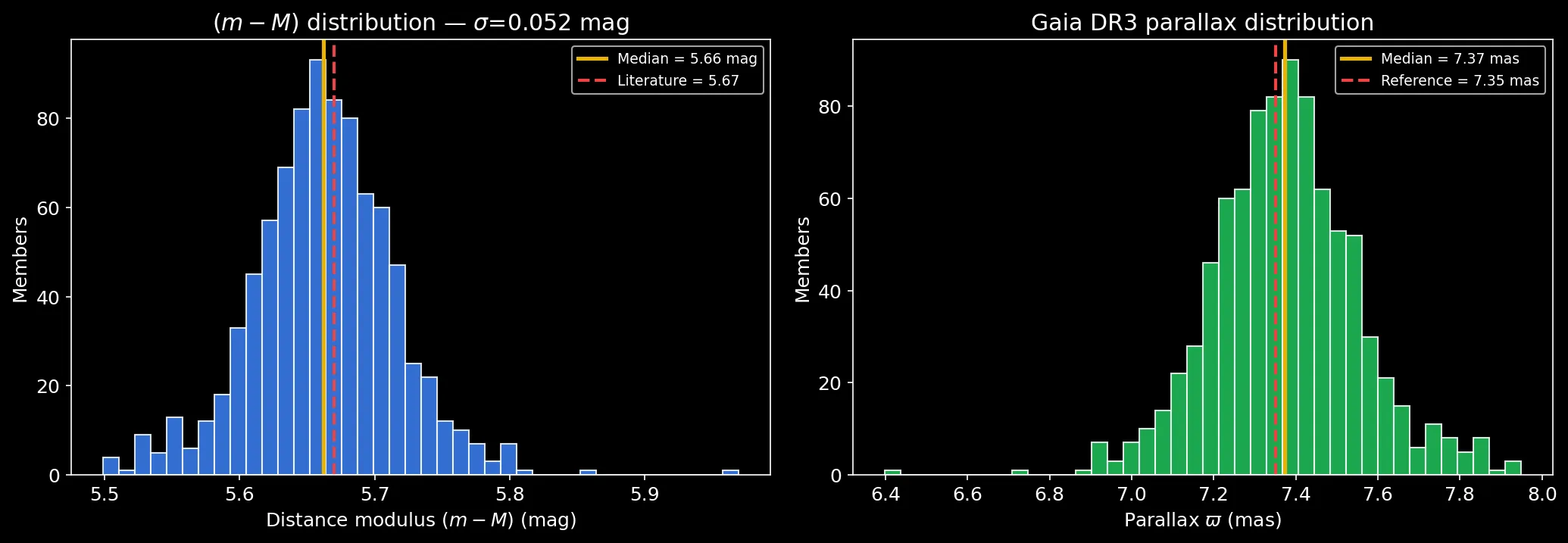
The distance modulus peaks at 5.66 mag, matching Babusiaux et al. (2018) at 5.67 ± 0.02. The parallax distribution centers on 7.37 mas, giving pc. Both are narrow and unimodal, confirming the member selection is clean. The slight asymmetry of the distance histogram is expected — is a non-linear transformation, so symmetric parallax errors become asymmetric in distance.
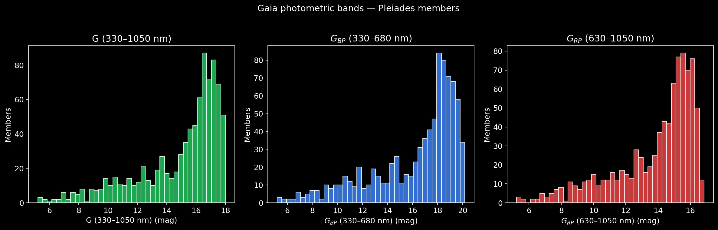
Gaia’s three bands
Gaia doesn’t observe in a single filter. It uses these three:
| Band | Wavelength | What it measures |
|---|---|---|
| G | 330–1050 nm (ultra-wide) | Total visible + near-IR flux |
| G_BP | 330–680 nm | Blue flux |
| G_RP | 630–1050 nm | Red flux |
The color index is a direct proxy for stellar temperature:
- → hot star (~10,000 K, type A, white-blue)
- → solar type (~5,800 K, type G, yellow)
- → cool star (~3,500 K, type M, red)
The physics is Wien’s displacement law: . A hotter star emits more blue photons → brighter in BP → smaller .
Other photometric systems exist, like Johnson-Cousins (U, B, V, R, I) from the 1950s, SDSS (u, g, r, i, z), and 2MASS (J, H, Ks) in the near-IR, but Gaia’s three bands cover 1.8 billion sources, so that’s what I’m working with.
Bolometric luminosity
A star radiates across the entire spectrum, not just the visible. The bolometric luminosity is the total power:
The dependence is steep: doubling the temperature gives 16× the luminosity. A bolometric correction bridges single-band magnitudes to bolometric: . For the Sun, (it emits mostly in the visible, so the correction is tiny). For an M dwarf, — the V band misses most of the flux because these stars peak in the infrared.
Building the CMD
The Color-Magnitude Diagram (CMD) is the observational counterpart of the HR diagram, arguably the most important single plot in stellar astrophysics.
- X-axis: → temperature (hot left, cool right)
- Y-axis: → luminosity (bright at top, faint at bottom — inverted axis)
I knew what to expect from textbooks, but seeing it emerge from real data was different. The features jumped out immediately:
- The main sequence (MS): the tight diagonal band where stars fuse hydrogen into helium. About 90% of a star’s life is spent here.
- The turn-off: where the most massive stars still on the MS are about to leave. Its position encodes the cluster age.
- M dwarfs (bottom-right): small, cool, faint. They dominate by number.
- A faint sequence about ~0.75 mag above the MS — unresolved binaries. Two equal-luminosity stars blended into one source: mag.
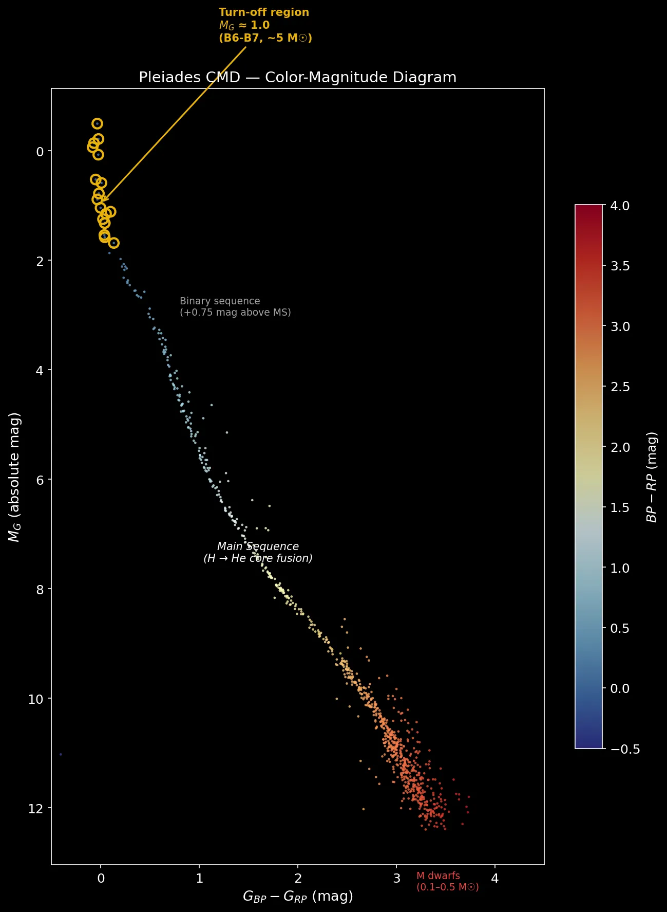
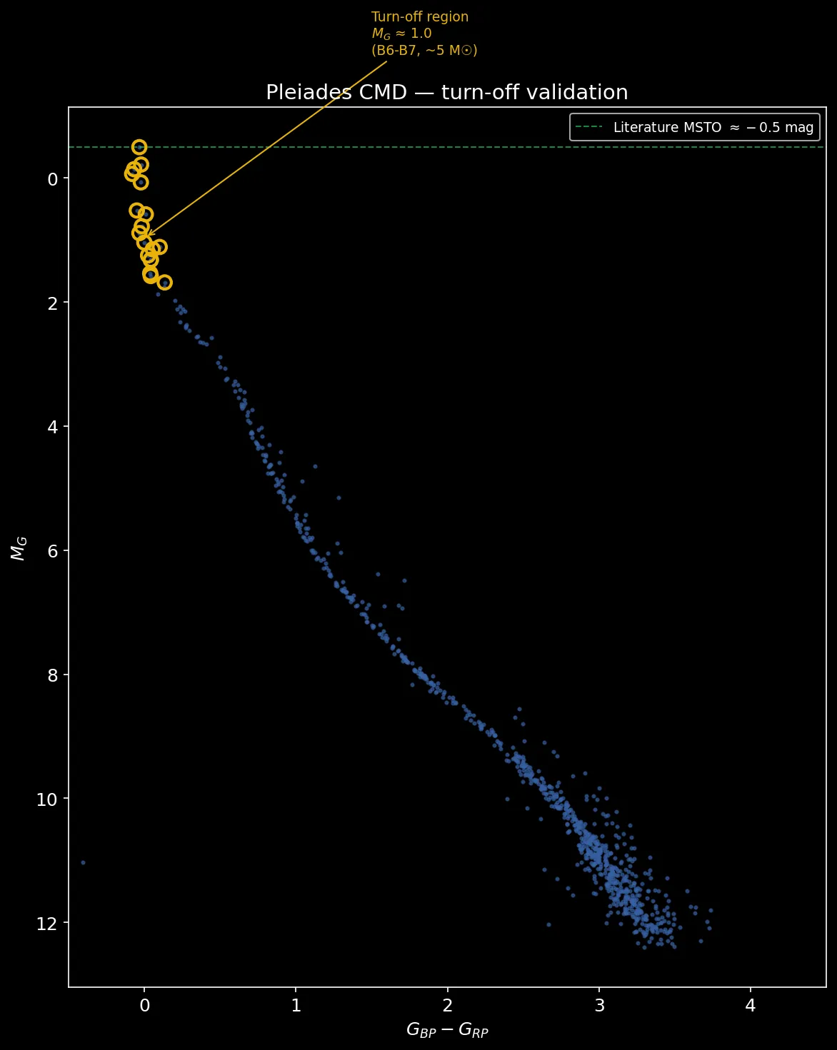
The Pleiades CMD is clean. Main sequence from bright B-type stars at the top-left down to faint M dwarfs at the bottom-right. The turn-off region sits near , , B6-B7 stars, about 5 . For a ~125 Myr cluster, that’s where it should be: every star more massive than this has already evolved off the main sequence.
The turn-off as a clock
The turn-off position is what makes CMDs powerful for dating clusters. The main-sequence lifetime scales roughly as yr, massive stars burn through their fuel much faster:
| Mass () | Type | (K) | MS lifetime |
|---|---|---|---|
| 0.5 | M | 3,800 | > 80 Gyr |
| 1.0 | G (Sun) | 5,780 | ~10 Gyr |
| 2.0 | A | 8,500 | ~1.5 Gyr |
| 5.0 | B | 15,000 | ~100 Myr |
| 10.0 | B | 28,000 | ~20 Myr |
In the Pleiades (~125 Myr), every star above ~5 has already left the main sequence. The turn-off sits at , . After the MS, the helium core contracts while the hydrogen envelope expands → the star moves onto the red giant branch (RGB): luminous but red, upper-right on the CMD. The Pleiades are too young to show a red giant branch — that’ll appear when I look at older clusters.
The key insight: the lower the turn-off on the CMD, the older the cluster. An older cluster (say, 625 Myr for the Hyades) would have its turn-off at , the A-type stars have run out of hydrogen. At 6.8 Gyr (NGC 188), even solar-type stars are leaving the MS, with the turn-off down at . Querying these clusters to see it for myself is on the list for a future post.
Apparent vs absolute CMD
I plotted both the apparent CMD ( vs , no distance correction) and the absolute CMD ( vs , corrected). For the Pleiades the difference is just a vertical shift of 5.67 mag, the shape is identical because all stars are at essentially the same distance.
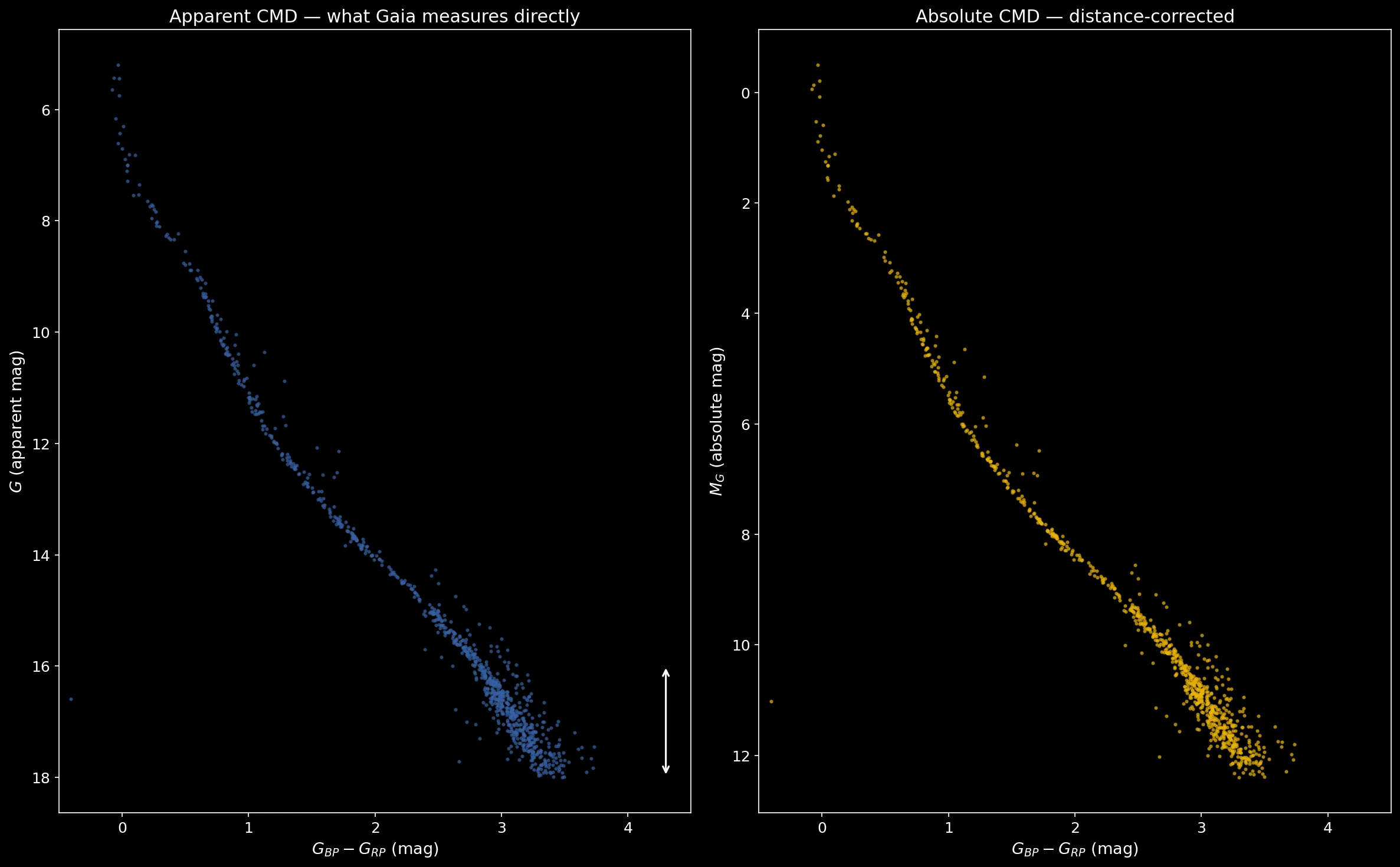
The absolute version is what you need when comparing clusters at different distances and they’ll overlap in . The apparent version is useful when fitting isochrones that you shift in distance modulus.
Uncertainties on the CMD
The CMD sequences aren’t infinitely thin. Part of the broadening is real, binaries, rotation, metallicity spread, but part is measurement noise so I wanted to see how much.
The full error propagation on absolute magnitude:
For the color index, both band errors add in quadrature: .
sigma_mG = np.sqrt(
    members['phot_g_mean_mag_error']**2 +
    (5/np.log(10))**2 * (members['parallax_error']/members['parallax'])**2
)
sigma_col = np.sqrt(
    members['phot_bp_mean_mag_error']**2 + members['phot_rp_mean_mag_error']**2
)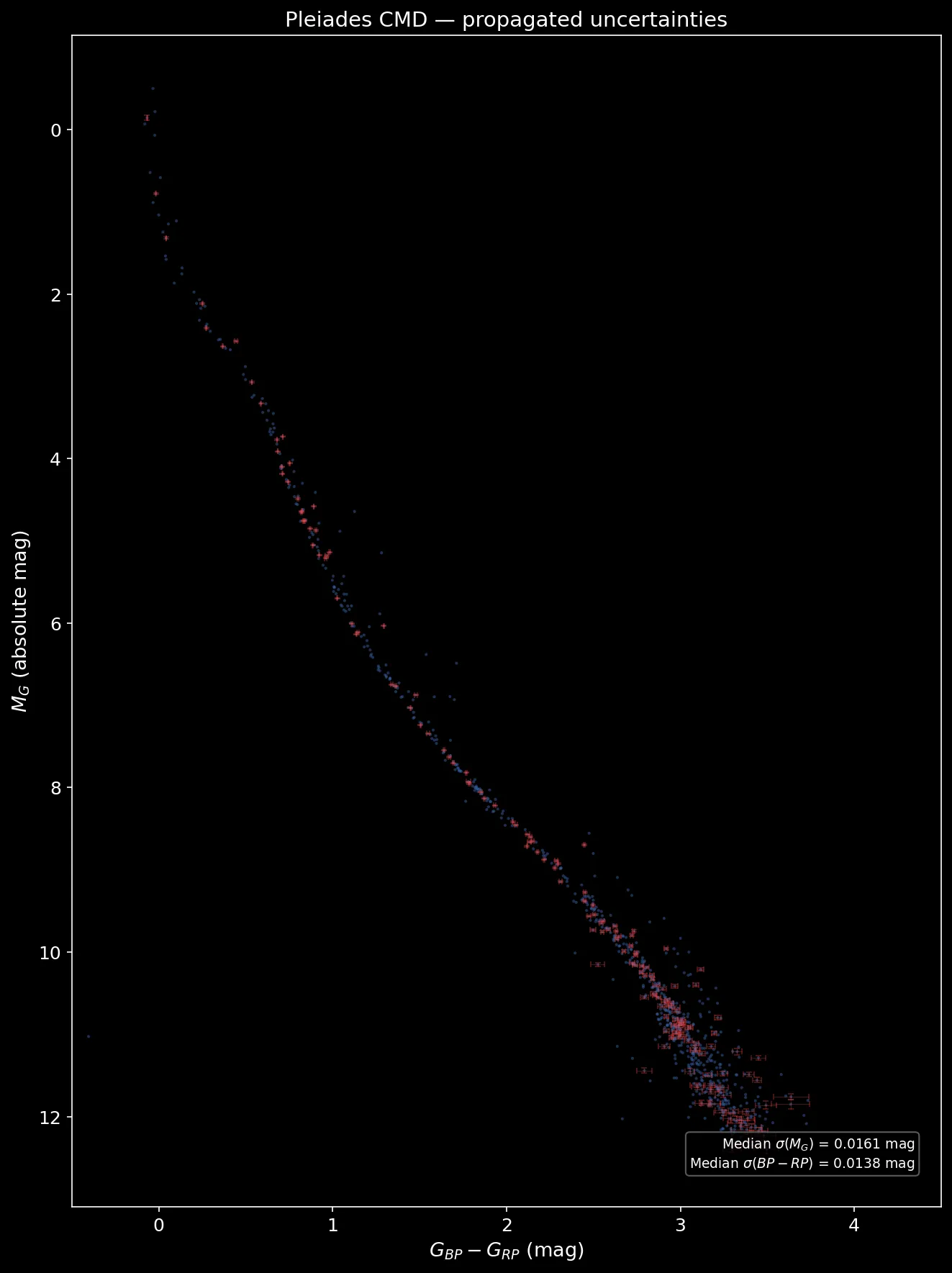
The median errors are tiny, mag, mag. The MS broadening is not measurement noise. It’s dominated by unresolved binaries (+0.75 mag for equal-mass pairs), differential reddening (minimal for the Pleiades), and possibly stellar rotation. For distant clusters behind the galactic plane, extinction would dwarf all of this, dust both dims and reddens starlight, shifting the entire CMD toward fainter and redder.
Validation
Same approach as the coordinates post, compare every derived quantity against published values:
| Quantity | My result | Literature | Match? |
|---|---|---|---|
| Distance (pc) | ~136 | 136 ± 1 | Ok |
| Distance modulus | 5.66 | 5.67 ± 0.02 | ok |
| Turn-off | ~−0.5 | ~−0.5 | ok |
| Members | ~870 | ~1000–1400 | Low but seems clean |
The member count is still lower than the literature, same reasons as the coordinates post: magnitude cut at and conservative proper motion radius miss the faintest and outermost members. But the derived physical quantities all match, which means the selection is clean if incomplete.
What’s next
- Try older clusters: the Hyades (~625 Myr) and NGC 188 (~6.8 Gyr) would show the turn-off dropping down the main sequence, a visual clock spanning billions of years
- Look at Isochrone fitting: overlay PARSEC/MIST theoretical models on the CMD to extract a precise age and metallicity. That’s where the CMD goes from qualitative to quantitative.
- Add dust corrections: apply dustmaps (SFD, Bayestar) to correct for extinction is essential for anything beyond ~500 pc or near the galactic plane, i should apply this
References
- Pogson (1856) — Magnitudes of Thirty-six of the Minor Planets. The original magnitude formalization.
- Bessell (2005) — Standard Photometric Systems. Annual Review of Astronomy and Astrophysics.
- Riello et al. (2021) — Gaia EDR3: Photometric content and validation. Gaia photometric system reference.
- Pecaut & Mamajek (2013) — Intrinsic Colors, Temperatures, and Bolometric Corrections of Pre-main-sequence Stars.
- Babusiaux et al. (2018) — Gaia DR2: Observational Hertzsprung-Russell diagrams. Gaia Collaboration.
- Bouy et al. (2015) — The Pleiades: the New 3D Structure from Gaia and Pan-STARRS1.